Analytical Instrument Calibration and Loop Integration: pH and Conductivity

Why analyzers get their own kind of attention

A pressure transmitter is mostly set and forget. Analytical sensors are not. The glass bulb on a pH electrode ages, coats over and slows down. A conductivity cell fouls. Neither one can be checked against a dial, only against chemistry: a buffer or a standard solution of known value. That is why plants calibrate them on a schedule, and why this is ordinary instrument technician work rather than something you do once at startup.

How a pH probe actually measures

A pH electrode is a small battery. The glass bulb develops a voltage that depends on the hydrogen ion activity of whatever it is sitting in: zero millivolts at pH 7, and about 59 mV for every pH unit away from that at 25 °C.

The catch is the "at 25 °C" part. That slope comes from the Nernst equation, and it scales with absolute temperature, so the same millivolt reading means a different pH in a cold sample than a warm one. That is why the probe carries a PT100 RTD and why we landed it on the transmitter's RTD terminals. The transmitter reads the temperature and corrects its slope continuously. Skip the RTD and the reading is only right at one temperature.

The loop

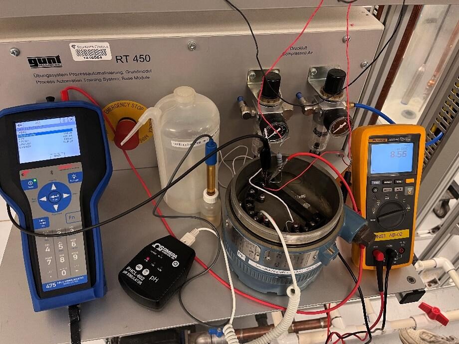
The 5081 is a two-wire transmitter, so the same pair of wires powers it and carries its signal. A 24 VDC supply, a 250 Ω resistor, the transmitter and the PLC's analog input channel all sit in one series loop. Whatever current the transmitter decides to pass, between 4 and 20 mA, is the signal.

The resistor is there for HART. HART rides a small digital signal on top of the 4 to 20 mA, and the communicator needs at least 250 Ω of loop resistance to see it. With the communicator clipped on, we set the range to 0.00 to 14.00 pH, so 4 mA means pH 0 and 20 mA means pH 14. A meter in series gave us an independent reading of the current, which matters later when you want to know whether a strange number is coming from the instrument or from the PLC.

Two calibrations, two different questions

We calibrated the pH transmitter twice, on purpose, because each method checks a different half of the instrument.

First, a pH simulator took the probe's place on the terminals and fed the transmitter a known millivolt signal. Using the HART communicator, we standardized at simulated pH 4.00 and 10.00 and used a third value to check. That proves the transmitter electronics and the loop, with the probe taken out of the picture entirely.

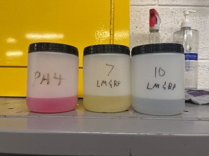
Then the probe went back in for a two-point buffer calibration. The pH 4 and pH 10 buffers set the two things that drift on a real electrode: the offset, which is where the line sits, and the slope, which is how many millivolts per pH the glass still produces. The pH 7 buffer was kept back as a check, and it read 7.09, inside 0.1 pH. The probe was rinsed with distilled water before every buffer, because a few drops of pH 10 carried into the pH 4 jar is enough to shift it, and each point was only accepted once the reading had stopped moving.

Doing both is how you find a fault quickly. If the simulator passes and the buffers fail, the problem is the probe. If both fail, look at the transmitter or the wiring.

Conductivity: setting the instrument up for the job

A conductivity sensor measures how easily current flows between two electrodes. The cell constant turns that into conductivity, and it decides which range the sensor is good for. The CDTX-2853 has a 1.0 cm⁻¹ cell, which covers roughly 10 to 10,000 µS/cm: tap water through to a fairly salty process stream, but not ultrapure water.

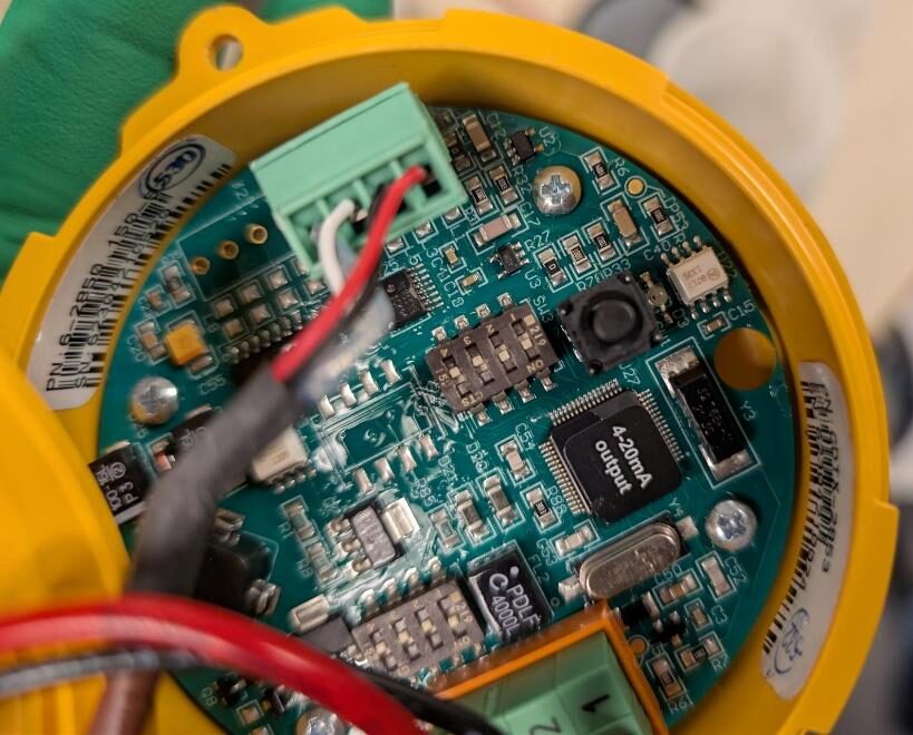
Its transmitter is configured with dip switches inside the housing. One bank sets the cell constant and turns on temperature compensation. Conductivity rises by roughly 2% for every degree Celsius, so without compensation a warm sample simply reads high. The other bank picks the span that gets mapped onto 4 to 20 mA. Our standards went up to 5000 µS/cm, so we set 0 to 5000.

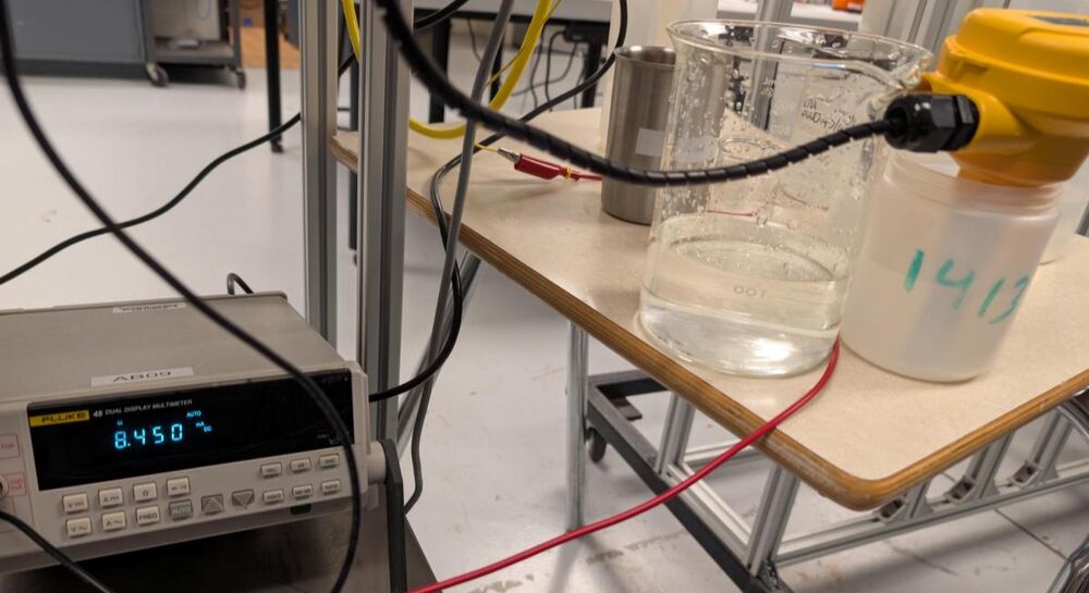
Before calibrating anything, we worked out what the loop should read. With 0 to 5000 µS/cm across 4 to 20 mA, the current is 4 + 16 × EC / 5000, so the 1413 µS/cm standard should give 8.52 mA and the 5000 µS/cm standard should give 20.00 mA. Writing the expected number down first means a bad reading is obvious the moment you see it.

Calibrating at one point, checking at another

This transmitter calibrates from a single standard. We reset it to factory calibration, put the probe in the 5000 µS/cm standard, shook it to knock off air bubbles, gave it two minutes to settle and held the calibration button until the LED cycled. The transmitter recognizes a standard within 10% of a value it knows and trims its output to match.

A reading of 20 mA in the 5000 standard after that says very little, because the calibration just forced it there. The real test was the 1413 µS/cm standard, which the calibration never saw. It read 8.61 mA against the 8.52 mA we predicted, a miss of about 28 µS/cm, or 0.55% of span.

For this instrument, the 24 VDC supply, a bench ammeter, the sensor and the PLC input were all wired in series, so there was always a second opinion on the current.

Turning current into a number the PLC can use

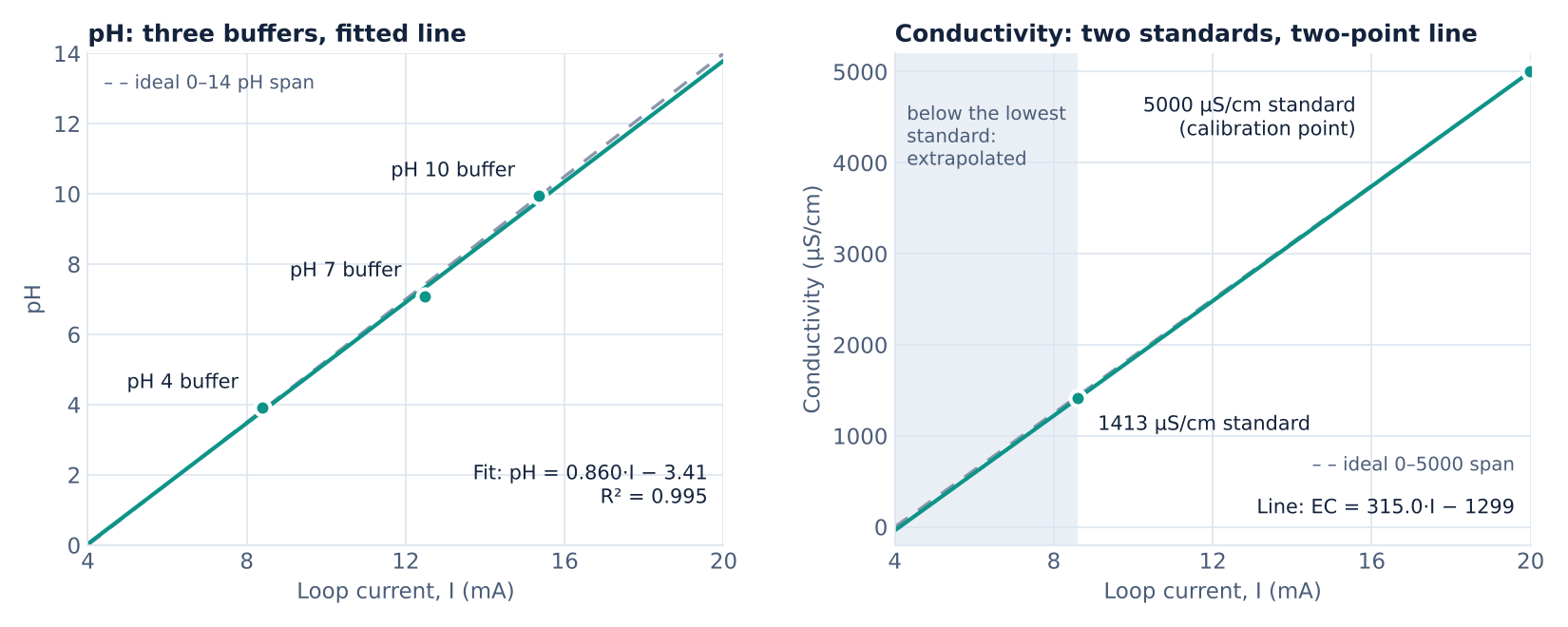
The PLC only receives current, so each instrument needed a scaling equation in ladder logic. For pH, we recorded the current and the HART reading in all three buffers and fitted a line through them: pH = 0.860 × I − 3.41 with I in milliamps, and an R² of 0.995. For conductivity, we drew a line through the two standards: EC = 315 × I − 1299 in milliamps.

The analog card had a surprise in it. It reported the conductivity loop in microamps, 8608 rather than 8.608, which we caught by looking at the raw tag before trusting anything downstream of it. The equation went into the PLC in microamps instead: EC = 0.315 × I − 1299.

Each program is two rungs. A MOV copies the raw analog channel into a REAL tag, and a CPT applies the scaling equation to produce the value the HMI displays.

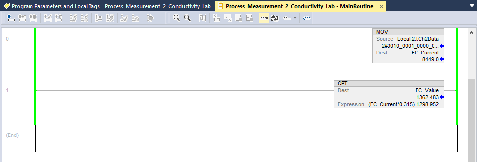
The handout had us derive the scaling from measured points, and it is a good way to see what the instrument is really doing. On a plant, I would scale straight from the configured range and use the HART communicator's loop trim to make the transmitter's current match its own reading. That way the PLC and the transmitter cannot end up disagreeing about the number.

Watching it respond

In FactoryTalk View, each value got a numeric display and a trend tied to the computed tag. The trends turned out to be the most interesting part of the whole exercise, because the two instruments behave nothing alike.

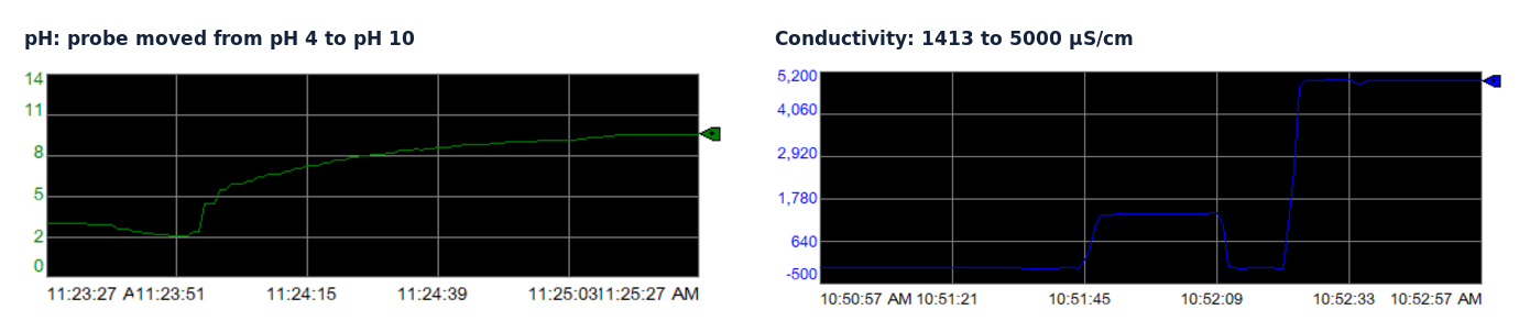
Moving the pH probe from the pH 4 buffer to pH 10 took about a minute and a half to settle, rinse included, and most of that was the last couple of pH units creeping in. Conductivity settled within five to ten seconds of each change, and most of that was us moving the probe. This matters if you ever have to tune a loop around one of these. A pH controller tuned as if its measurement were instant will chase the slow tail of the electrode and oscillate. Knowing how long the sensor takes is part of the tuning.

Where the numbers stopped being trustworthy

• Distilled water read −30 µS/cm, which cannot happen. It is what the line gives when you extend it below the lowest standard, where it reaches about −39 µS/cm at 4 mA. Distilled water is also below the 10 µS/cm floor of a 1.0 cell to begin with. The fix is a third standard near 100 µS/cm, or a 0.1 cell if pure water is the actual job. Clamping the tag at zero would hide the number without fixing the error, so we left it showing.
• The recheck in the 1413 standard read 1362 µS/cm, about 3.5% low. Since the meter and the PLC agreed on the current, the difference sits on the sensor side: tap water left on the probe from rinsing, bubbles, a shorter wait or a different sample temperature. Next time I would rinse with a splash of the next standard, take several readings per standard and log the temperature.
• As set up, the conductivity loop is good from roughly 1400 to 5000 µS/cm. Anything below that needs more calibration before anyone acts on it.